Background
In this post, I’m going to train a machine learning model to predict mobile phone price from this Kaggle dataset.
The task is as follows: given a phone’s specifications (e.g. RAM, number of processors, camera resolution, etc.), predict the phone price range (low, medium, high, or very high).
There are several different approaches here compared to the one I used on my previous post:
- Data preprocessing: instead of defining my own functions to fit and transform the data, I used the
make_pipelinefunction from scikit learn, which makes the task much more convenient. - Model selection: instead of running a grid search on each model, I just use the default hyperparameters, then run the grid search on the best model. This is because running grid search on each model takes a really long time. I also use k-fold cross validation here instead of evaluating the data on the validation set.
Loading the Modules
import pandas as pd
import numpy as np
import matplotlib.pyplot as plt
import seaborn as sns

from sklearn.preprocessing import StandardScaler
from sklearn.model_selection import train_test_split, cross_val_score, GridSearchCV
from sklearn.pipeline import make_pipeline
from sklearn.metrics import accuracy_score

from sklearn.linear_model import LogisticRegression
from sklearn.tree import DecisionTreeClassifier
from sklearn.dummy import DummyClassifier
from sklearn.ensemble import RandomForestClassifier, AdaBoostClassifier, BaggingClassifier, GradientBoostingClassifier
from sklearn.svm import SVC
from sklearn.discriminant_analysis import LinearDiscriminantAnalysis
from sklearn.metrics import confusion_matrix, classification_report, ConfusionMatrixDisplay
Loading the Data
df = pd.read_csv('./data/train.csv')
print('Data shape:', df.shape)
df.head()
Output:
Data shape: (2000, 21)
| battery_power | blue | clock_speed | dual_sim | fc | four_g | int_memory | m_dep | mobile_wt | n_cores | … | px_height | px_width | ram | sc_h | sc_w | talk_time | three_g | touch_screen | wifi | price_range | |
|---|---|---|---|---|---|---|---|---|---|---|---|---|---|---|---|---|---|---|---|---|---|
| 0 | 842 | 0 | 2.2 | 0 | 1 | 0 | 7 | 0.6 | 188 | 2 | … | 20 | 756 | 2549 | 9 | 7 | 19 | 0 | 0 | 1 | 1 |
| 1 | 1021 | 1 | 0.5 | 1 | 0 | 1 | 53 | 0.7 | 136 | 3 | … | 905 | 1988 | 2631 | 17 | 3 | 7 | 1 | 1 | 0 | 2 |
| 2 | 563 | 1 | 0.5 | 1 | 2 | 1 | 41 | 0.9 | 145 | 5 | … | 1263 | 1716 | 2603 | 11 | 2 | 9 | 1 | 1 | 0 | 2 |
| 3 | 615 | 1 | 2.5 | 0 | 0 | 0 | 10 | 0.8 | 131 | 6 | … | 1216 | 1786 | 2769 | 16 | 8 | 11 | 1 | 0 | 0 | 2 |
| 4 | 1821 | 1 | 1.2 | 0 | 13 | 1 | 44 | 0.6 | 141 | 2 | … | 1208 | 1212 | 1411 | 8 | 2 | 15 | 1 | 1 | 0 | 1 |
Below are the definitions of each variable, according to the the Kaggle page:
battery_power: Total energy a battery can store in one time measured in mAhblue: Has bluetooth or notclock_speed: Speed at which microprocessor executes instructionsdual_sim: Has dual sim support or notfc: Front Camera mega pixelsfour_g: Has 4G or notint_memory: Internal Memory in Gigabytesm_dep: Mobile Depth in cmmobile_wt: Weight of mobile phonen_cores: Number of cores of processorpc: Primary Camera mega pixelspx_height: Pixel Resolution Heightpx_width: Pixel Resolution Widthram: Random Access Memory in Mega Bytessc_h: Screen Height of mobile in cmsc_w: Screen Width of mobile in cmtalk_time: Longest time that a single battery charge will last when you arethree_g: Has 3G or nottouch_screen: Has touch screen or notwifi: Has wifi or notprice_range: This is the target variable with value of 0 (low cost), 1 (medium cost), 2 (high cost) and 3 (very high cost).
Checking each variable’s type:
df.info()
Output:
<class 'pandas.core.frame.DataFrame'>
RangeIndex: 2000 entries, 0 to 1999
Data columns (total 21 columns):
 #   Column         Non-Null Count  Dtype
---  ------         --------------  -----
 0   battery_power  2000 non-null   int64
 1   blue           2000 non-null   int64
 2   clock_speed    2000 non-null   float64
 3   dual_sim       2000 non-null   int64
 4   fc             2000 non-null   int64
 5   four_g         2000 non-null   int64
 6   int_memory     2000 non-null   int64
 7   m_dep          2000 non-null   float64
 8   mobile_wt      2000 non-null   int64
 9   n_cores        2000 non-null   int64
 10  pc             2000 non-null   int64
 11  px_height      2000 non-null   int64
 12  px_width       2000 non-null   int64
 13  ram            2000 non-null   int64
 14  sc_h           2000 non-null   int64
 15  sc_w           2000 non-null   int64
 16  talk_time      2000 non-null   int64
 17  three_g        2000 non-null   int64
 18  touch_screen   2000 non-null   int64
 19  wifi           2000 non-null   int64
 20  price_range    2000 non-null   int64
dtypes: float64(2), int64(19)
memory usage: 328.3 KB
Checking for missing values:
df.isnull().sum()
Output:
battery_power    0
blue             0
clock_speed      0
dual_sim         0
fc               0
four_g           0
int_memory       0
m_dep            0
mobile_wt        0
n_cores          0
pc               0
px_height        0
px_width         0
ram              0
sc_h             0
sc_w             0
talk_time        0
three_g          0
touch_screen     0
wifi             0
price_range      0
dtype: int64
Finding out which variables are binary (only have 2 unique values):
df.apply(lambda col: col.nunique(), axis=0).sort_values()
Output:
blue                2
touch_screen        2
dual_sim            2
four_g              2
three_g             2
wifi                2
price_range         4
n_cores             8
m_dep              10
sc_h               15
talk_time          19
sc_w               19
fc                 20
pc                 21
clock_speed        26
int_memory         63
mobile_wt         121
battery_power    1094
px_width         1109
px_height        1137
ram              1562
dtype: int64
Defining the binary variables:
bin_vars = ['blue', 'touch_screen', 'dual_sim', 'four_g', 'three_g', 'wifi']
Train/Test Split
The data consist of 2000 rows, which is not a lot. So I’m just going to split the data into two sets: the training set and the test set. To choose the best model, later on I’m going to use K-fold cross-validation.
df_train, df_test = train_test_split(df, test_size=0.3, random_state=112)
Exploratory Data Analysis
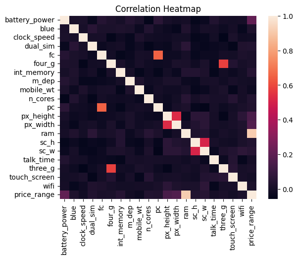
Correlation Heatmap
sns.heatmap(df_train.corr())
plt.title('Correlation Heatmap')
Target Variable Distribution
sns.countplot(df_train, y='price_range')
plt.title('Target Variable Distribution')
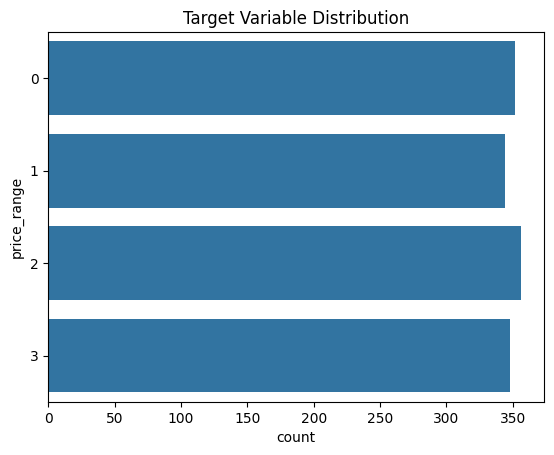
Observation: the target variable seems to be well-balanced.
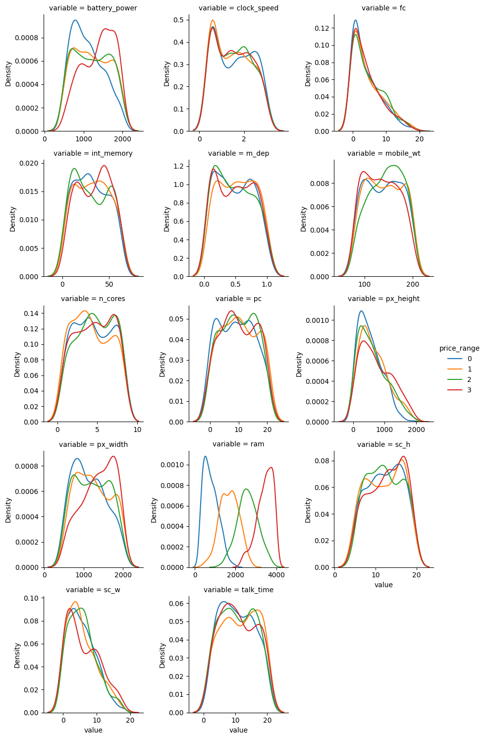
Numerical Variable Distributions
df_long = df_train.melt(id_vars='price_range')
is_bin_vars = df_long['variable'].isin(bin_vars)
df_long_num = df_long[~is_bin_vars]
df_long_cat = df_long[is_bin_vars]

g = sns.FacetGrid(df_long_num, col='variable', hue='price_range', col_wrap=3, sharex=False, sharey=False)
g.map_dataframe(sns.kdeplot, x='value')
g.add_legend()
sns.catplot(df_long_num, kind='box',
            col='variable', col_wrap=3,
            x='price_range', y='value',
            sharex=False, sharey=False)
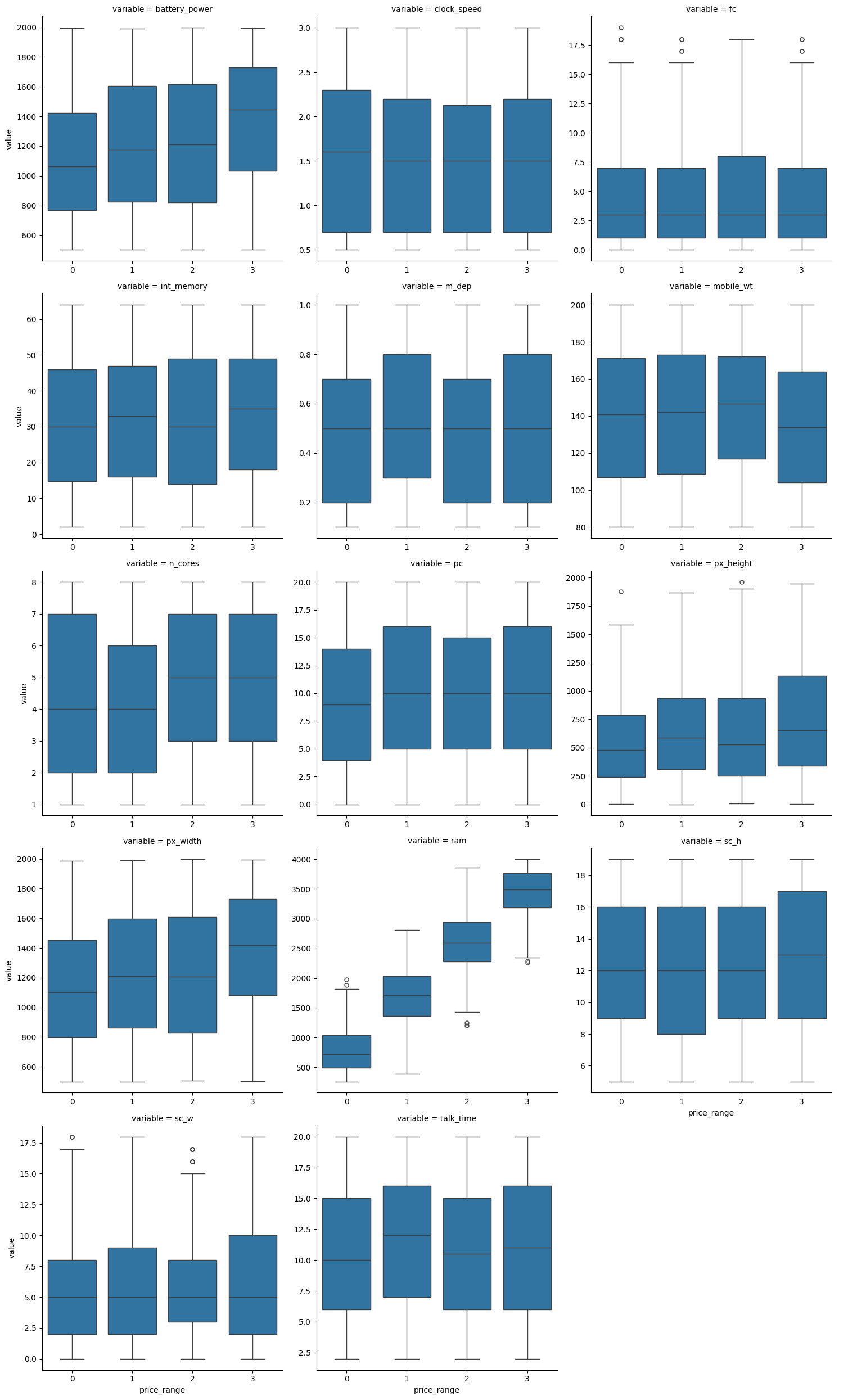
Observation: only ram variable shows a linear relationship with the price range (more expensive phone tends to have higher RAM).
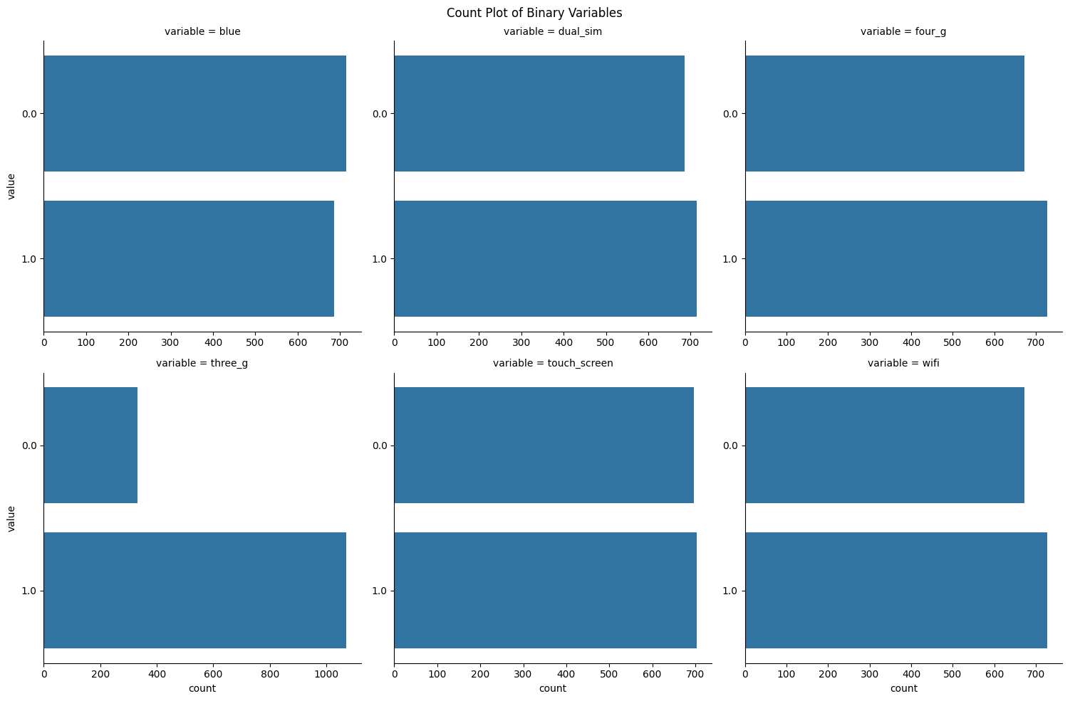
Binary Variable Distributions
g = sns.catplot(df_long_cat, kind='count',
            col='variable', col_wrap=3,
            y='value',
            sharex=False, sharey=False)
g.fig.suptitle('Count Plot of Binary Variables')
plt.tight_layout()
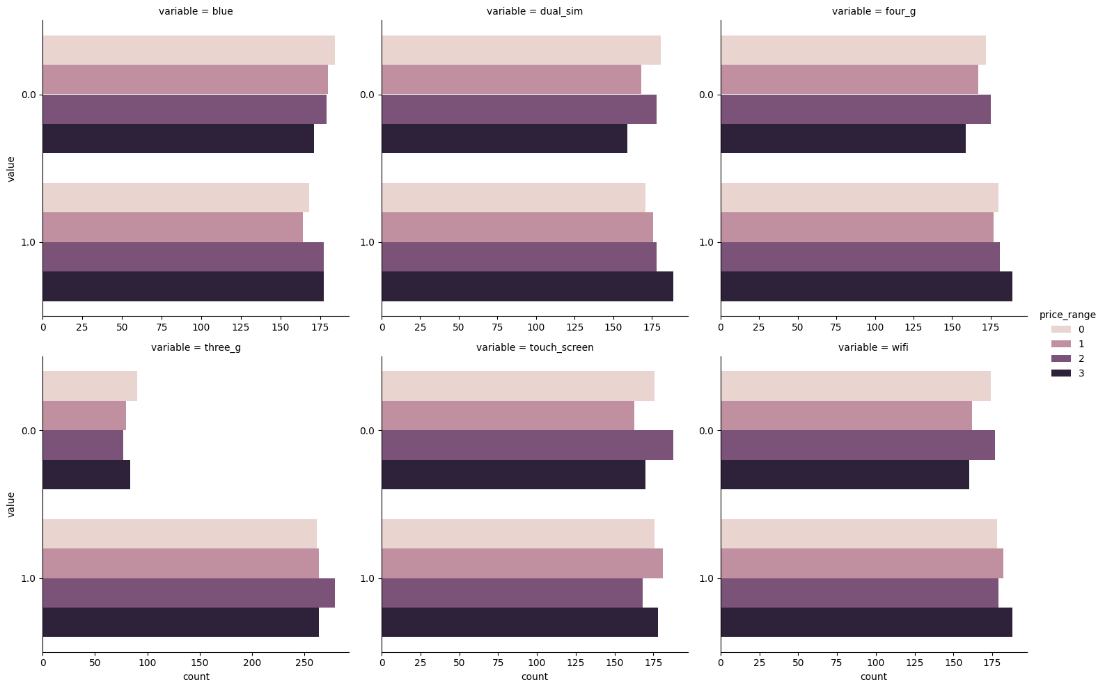
sns.catplot(df_long_cat, kind='count',
            col='variable', col_wrap=3,
            y='value', hue='price_range',
            sharex=False, sharey=False)
EDA Conclusions
- There is no categorical columns, so we don’t need to do any encoding
- There is no missing/invalid values, so we don’t need to do any imputing
- There is no outliers, so we don’t need to do any outlier treatment
- So far there’s no feature-engineering that we can do
X/Y Split
def split_X_y(df: pd.DataFrame, target_col: str, feature_cols: list[str]) -> tuple[pd.DataFrame, pd.Series]:
    return (
        df[feature_cols],
        df[target_col]
    )

target_col = 'price_range'
feature_cols = df_train.columns.drop(target_col)

X_train, y_train = split_X_y(df_train, target_col, feature_cols)
X_test, y_test = split_X_y(df_test, target_col, feature_cols)

print('Train shape:', X_train.shape)
print('Test shape:', X_test.shape)
Output:
Train shape: (1400, 20)
Test shape: (600, 20)
Modeling
In this section, I’m going to train several machine learning models.
For preprocessing, I’m only going to standardize the values, and I’m going to make use of the make_pipeline function.
Moreover, since there’s no validation data set, I’m just going to use k-fold cross validation to determine the “out-of-sample” performance.
%%time

models = {
    'Dummy Classifier': DummyClassifier(),
    'Logistic Regression': LogisticRegression(random_state=519),
    'Decision Tree': DecisionTreeClassifier(random_state=882),
    'Random Forest': RandomForestClassifier(random_state=511),
    'Bagging': BaggingClassifier(random_state=112),
    'Ada Boost': AdaBoostClassifier(random_state=919, algorithm='SAMME'),
    'Gradient Boosting': GradientBoostingClassifier(random_state=114),
    'LDA': LinearDiscriminantAnalysis(),
    'SVC': SVC(),
}

model_pipelines = {}
model_scores = {}

for model_name, model in models.items():
    model_pipeline = make_pipeline(
        StandardScaler(),
        model
    )
    scores = cross_val_score(
        model_pipeline,
        X_train, y_train,
        cv=5, scoring='accuracy'
    )

    model_pipeline.fit(X_train, y_train)
    model_pipelines[model_name] = model_pipeline

    model_scores[model_name] = scores.mean()
Output:
CPU times: total: 23 s
Wall time: 23.7 s
Let’s compare the out-of-sample performance of each model:
model_scores_df = (pd.Series(model_scores)
                   .sort_values()
                   .reset_index()
                   .set_axis(['Model', 'Score'], axis=1))
model_scores_df
| Model | Score | |
|---|---|---|
| 0 | Dummy Classifier | 0.254286 |
| 1 | Ada Boost | 0.488571 |
| 2 | Decision Tree | 0.816429 |
| 3 | SVC | 0.862857 |
| 4 | Bagging | 0.865000 |
| 5 | Random Forest | 0.873571 |
| 6 | Gradient Boosting | 0.892857 |
| 7 | LDA | 0.942143 |
| 8 | Logistic Regression | 0.946429 |
Based on the result above, we have to conclude that the logistic regression model is the best one with accuracy of 94.6%. Next, I’m going to tune the model’s hyperparameter using grid search.
Hyperparameter Tuning
%%time

lr_grid = GridSearchCV(
    make_pipeline(StandardScaler(), LogisticRegression()),
    param_grid={
        'logisticregression__C': np.logspace(-5, 3, 20),
    },
    cv=5,
    scoring='accuracy'
)
lr_grid.fit(X_train, y_train)

print('Best model parameters:', lr_grid.best_params_)
print('Best model score:', lr_grid.best_score_)
Output:
Best model parameters: {'logisticregression__C': 54.555947811685144}
Best model score: 0.9657142857142856
CPU times: total: 2.86 s
Wall time: 2.92 s
As you can see, by running a grid search we’ve managed to improve the accuracy from 94.6% to 96.6%.
Model Evaluation
Now let’s evaluate the model on the test data.
best_model = lr_grid.best_estimator_

y_train_pred = best_model.predict(X_train)
y_test_pred = best_model.predict(X_test)

test_accuracy = accuracy_score(y_test, y_test_pred)

print('Test accuracy:', test_accuracy)
Output:
Test accuracy: 0.965
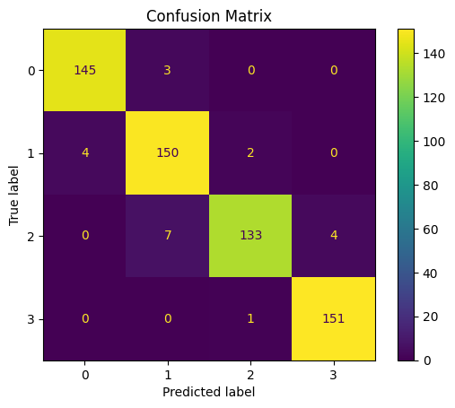
test_confusion_matrix = ConfusionMatrixDisplay(
    confusion_matrix(y_test, y_test_pred),
    display_labels=best_model.classes_
)
test_confusion_matrix.plot()
plt.title('Confusion Matrix')
plt.show()
print(classification_report(y_test, y_test_pred))
Output:
              precision    recall  f1-score   support

           0       0.97      0.98      0.98       148
           1       0.94      0.96      0.95       156
           2       0.98      0.92      0.95       144
           3       0.97      0.99      0.98       152

    accuracy                           0.96       600
   macro avg       0.97      0.96      0.96       600
weighted avg       0.97      0.96      0.96       600
Overall, our model seems to work well on the test data, achieving 96% accuracy and 96% average F1 score.
It is also worth noting that the misclassified cases are still only 1 notch away from the true price range (which is good):
y_test_diff = (y_test_pred - y_test)
y_test_diff.value_counts()
Output:
price_range
 0    579
-1     12
 1      9
Name: count, dtype: int64
Conclusion
That’s it for this post. I hope you learning something new today.