Background
In this post, I’m going to share how I trained a machine learning model to predict bank customer churn (i.e. customers that stop doing business with the bank) using data from this Kaggle page. Why is this kind of task important? Typically, the cost of acquiring a new customer is much more expensive than the cost of retaining a customer. And so, it is in the company’s best interest to retain its customers for as long as possible. By accurately knowing which customers are likely to churn, the company can give those customers some treatment intended to prevent them from churning.
I’m going to use Python to do this exercise.
Loading Modules & Defining Some Functions
In this section, I’m going to load all the Python modules & define some functions that I’m going to use. Feel free to skip ahead to the next section.
Loading Modules
from datetime import datetime
import pandas as pd
import numpy as np
import matplotlib.pyplot as plt
import seaborn as sns
from sklearn.model_selection import train_test_split
from sklearn.preprocessing import OneHotEncoder
from sklearn.linear_model import LogisticRegression
from sklearn.impute import SimpleImputer
from sklearn.preprocessing import StandardScaler

from sklearn.tree import DecisionTreeClassifier
from sklearn.model_selection import GridSearchCV
from sklearn.linear_model import LogisticRegression
from sklearn.ensemble import GradientBoostingClassifier, BaggingClassifier
from sklearn.dummy import DummyClassifier
from sklearn.neural_network import MLPClassifier
from sklearn.base import BaseEstimator

from sklearn.metrics import roc_auc_score, f1_score, accuracy_score
from typing import Any
Defining Helper Functions
For Exploratory Data Analysis
def create_subplots_grid(n_vars: int, ncols: int) -> tuple[plt.Figure, np.ndarray]:
    '''
    Create subplots fig & axes for creating subplots

    Parameters
    ----------
    n_vars : int
        Number of plots you want to create
    ncols : int
        Number of plot columns you want to create

    Returns:
    --------
    fig : plt.Figure
    axes : list of flatten axes
    '''
    nrows = int(np.ceil(n_vars / ncols))
    fig, axes = plt.subplots(nrows=nrows, ncols=ncols)
    axes = axes.flatten()
    return (fig, axes)
For Data Preprocessing
def fit_imputer(
    df: pd.DataFrame,
    num_cols: list[str],
    cat_cols: list[str]
) -> tuple[SimpleImputer, SimpleImputer]:
    '''
    Fit missing data imputer for numerical and categorical variables.

    Parameters
    ----------
    df : pd.DataFrame
    num_cols : list of str
        Name of numerical variables
    cat_cols : list of str
        Name of categorical variables

    Returns
    -------
    num_imputer : SimpleImputer
        Imputer for numerical variables
    cat_imputer : SimpleImputer
        Imputer for categorical variables
    '''
    num_imputer = SimpleImputer(strategy='mean')
    num_imputer.fit(df[num_cols])
    cat_imputer = SimpleImputer(strategy='most_frequent')
    cat_imputer.fit(df[cat_cols])
    return num_imputer, cat_imputer

def impute_data(
    df: pd.DataFrame,
    num_imputer: SimpleImputer,
    cat_imputer: SimpleImputer
) -> pd.DataFrame:
    '''
    Transform the given dataframe with the given imputers.

    Parameters
    ----------
    df : pd.DataFrame
    num_imputer : SimpleImputer object
    cat_imputer : SimpleImputer object

    Returns
    -------
    df : pd.DataFrame
        Data where the relevant columns have been imputed.
    '''
    df = df.copy()
    num_cols = num_imputer.feature_names_in_
    cat_cols = cat_imputer.feature_names_in_
    df[num_cols] = num_imputer.transform(df[num_cols])
    df[cat_cols] = cat_imputer.transform(df[cat_cols])
    return df

def fit_ohe(df: pd.DataFrame, cat_cols: list[str]) -> OneHotEncoder:
    '''
    Fit one-hot encoder for the categorical columns

    Parameters
    ----------
    df : pd.DataFrame
    cat_cols : list of str
        Name of categorical columns

    Returns
    -------
    ohe : OneHotEncoder object
    '''
    ohe = OneHotEncoder(drop='if_binary', handle_unknown='ignore', sparse_output=False)
    ohe.fit(df[cat_cols])
    return ohe

def transform_ohe(df: pd.DataFrame, ohe: OneHotEncoder) -> pd.DataFrame:
    '''
    Transform the categorical columns using one-hot encoder

    Parameters
    ----------
    df : pd.DataFrame
    ohe : fitted OneHotEncoder object

    Returns
    -------
    df_ohe : pd.DataFrame
        Dataframe with categorical variables
        transformed using one-hot encoder.
    '''
    cat_cols = ohe.feature_names_in_
    df = df.copy()
    df_ohe = pd.DataFrame(
        ohe.transform(df[cat_cols]),
        index=df.index,
        columns=ohe.get_feature_names_out()
    )
    df = pd.concat([df, df_ohe], axis=1)
    df = df.drop(cat_cols, axis=1)
    return df

def fit_scaler(df: pd.DataFrame) -> StandardScaler:
    '''
    Fit a standard scaler on all columns

    Parameters
    ----------
    df : pd.DataFrame

    Returns
    -------
    scaler : StandardScaler object
    '''
    scaler = StandardScaler()
    scaler.fit(df)
    return scaler

def transform_scaler(df: pd.DataFrame, scaler: StandardScaler) -> pd.DataFrame:
    '''
    Transform data using a standard scaler

    Parameters
    ----------
    df : pd.DataFrame
    scaler : fitted StandardScaler object

    Returns
    -------
    df_out : pd.DataFrame
    '''
    df_out = pd.DataFrame(
        scaler.transform(df),
        index=df.index,
        columns=df.columns
    )
    return df_out

def preprocess_data(
    df: pd.DataFrame,
    num_imputer: SimpleImputer,
    cat_imputer: SimpleImputer,
    ohe: OneHotEncoder,
    scaler: StandardScaler,
    feature_cols: list[str],
    target_col: str
) -> tuple[pd.DataFrame, pd.Series]:
    '''
    Preprocess data from start to finish.

    Parameters
    ----------
    df : pd.DataFrame
    num_imputer : SimpleImputer
    cat_imputer : SimpleImputer
    ohe : OneHotEncoder
    scaler : StandardScaler
    feature_cols : list of str
    target_col : str

    Returns
    -------
    X : pd.DataFrame
    y : pd.Series
    '''
    df = df.copy()
    df = impute_data(df, num_imputer, cat_imputer)
    df = transform_ohe(df, ohe)
    X = df[feature_cols]
    X = transform_scaler(X, scaler)
    y = df[target_col]
    return (X, y)
For Training Models
def calc_metrics(model: BaseEstimator, X: pd.DataFrame, y: pd.Series) -> dict[str, float]:
    y_pred = model.predict(X)
    y_pred_prob = model.predict_proba(X)[:, 1]
    return {
        'f1': f1_score(y, y_pred),
        'roc_auc': roc_auc_score(y, y_pred_prob),
        'accuracy': accuracy_score(y, y_pred),
    }

def fit_eval_cv(
    cv_obj: GridSearchCV,
    X_train: pd.DataFrame,
    y_train: pd.Series,
    X_test: pd.DataFrame,
    y_test: pd.Series
) -> dict[str, Any]:
    '''
    Fit and evaluate the given cv model.
    Will print out the train/test scores.
    Returns dictionary containing:
    - training_score
    - test_score
    - best_model
    - best_params
    '''
    start_time = datetime.now()
    cv_obj.fit(X_train, y_train)
    elapsed = datetime.now() - start_time
    print(f'Elapsed: {elapsed}')

    test_score = cv_obj.score(X_test, y_test)
    best_params = cv_obj.best_params_
    best_model = cv_obj.best_estimator_

    print(f'Valid score: {test_score:.4f}')
    print(f'Best Params: {best_params}')
    return {
        'test_score': test_score,
        'best_model': best_model,
        **calc_metrics(best_model, X_test, y_test)
    }
Exploratory Data Analysis (EDA)
Some basic properties
Let’s load the data and examine some of its properties.
df = pd.read_csv('./data/Churn_Modelling.csv')
df.head()
| RowNumber | CustomerId | Surname | CreditScore | Geography | Gender | Age | Tenure | Balance | NumOfProducts | HasCrCard | IsActiveMember | EstimatedSalary | Exited | |
|---|---|---|---|---|---|---|---|---|---|---|---|---|---|---|
| 0 | 1 | 15634602 | Hargrave | 619 | France | Female | 42 | 2 | 0 | 1 | 1 | 1 | 101348.9 | 1 |
| 1 | 2 | 15647311 | Hill | 608 | Spain | Female | 41 | 1 | 83807.86 | 1 | 0 | 1 | 112542.6 | 0 |
| 2 | 3 | 15619304 | Onio | 502 | France | Female | 42 | 8 | 159660.8 | 3 | 1 | 0 | 113931.6 | 1 |
| 3 | 4 | 15701354 | Boni | 699 | France | Female | 39 | 1 | 0 | 2 | 0 | 0 | 93826.63 | 0 |
| 4 | 5 | 15737888 | Mitchell | 850 | Spain | Female | 43 | 2 | 125510.8 | 1 | NaN | 1 | 79084.1 | 0 |
The data has several columns that I definitely don’t need for making predictions: RowNumber, CustomerId, and Surname, so I will remove them from the data:
df_dropped_cols = df.drop(['RowNumber', 'CustomerId', 'Surname'], axis=1)
In doing exploratory data analysis, it is important not to look at the validation & test set, and so I will split the data set into three parts:
- Training set: this is the one that I’m going to use for EDA & for training the models.
- Validation set: this is for measuring out-of-sample performance of each model. The model with the highest performance will be picked.
- Test set: this is for last performance evaluation. I have to make sure that the model still works on truly out-of-sample data.
print('Full data shape:', df_dropped_cols.shape)

df_train, df_non_train = train_test_split(df_dropped_cols, test_size=0.2, random_state=4123)
df_valid, df_test = train_test_split(df_non_train, test_size=0.5, random_state=5101)

print('Training data shape:', df_train.shape)
print('Validation data shape:', df_valid.shape)
print('Test data shape:', df_test.shape)
Output:
Full data shape: (10002, 11)
Training data shape: (8001, 11)
Validation data shape: (1000, 11)
Test data shape: (1001, 11)
df_train.head()
| CreditScore | Geography | Gender | Age | Tenure | Balance | NumOfProducts | HasCrCard | IsActiveMember | EstimatedSalary | Exited | |
|---|---|---|---|---|---|---|---|---|---|---|---|
| 7235 | 697 | France | Male | 35 | 5 | 133087.8 | 1 | 1 | 0 | 64771.61 | 0 |
| 2427 | 798 | Germany | Female | 49 | 5 | 132571.7 | 1 | 1 | 1 | 31686.33 | 1 |
| 1207 | 752 | Germany | Male | 30 | 4 | 81523.38 | 1 | 1 | 1 | 36885.85 | 0 |
| 2948 | 620 | France | Female | 29 | 1 | 138740.2 | 2 | 0 | 0 | 154700.6 | 0 |
| 6990 | 660 | France | Male | 41 | 3 | 0 | 2 | 1 | 1 | 108665.9 | 0 |
The complete data set has about ten thousand rows, which is good enough for training an ML model. In the data, each row corresponds to a customer, and each column corresponds to the property of each customer (to see the definitions of each column, the reader is referred to the Kaggle page). The target variable that I need to predict is the Exited column, where the value is 1 if the customer churned, and 0 if the customer didn’t churn.
What is the overall churn rate of this company?
df_train['Exited'].mean()
Output:
0.20497437820272466
As it turns out, there’s about 20% of churning customers.
Data distributions
Next, let’s see the distribution of the data using histogram. I will use different plots for categorical and numerical columns.
Below I’m defining which columns are categorical and which are numerical:
target_col = 'Exited'
cat_cols = ['Geography', 'Gender', 'HasCrCard', 'IsActiveMember', 'NumOfProducts']
num_cols = ['CreditScore', 'Age', 'Tenure', 'Balance', 'EstimatedSalary']
The column NumOfProducts sounds like it should be a numeric column. However, as we’ll see later, I believe it’s better to treat it as a categorical column, because that column only has four unique values, and the class distribution is very imbalanced.
Numerical variables distributions
Below is the histogram for each numerical variables:
fig, axes = create_subplots_grid(len(num_cols), ncols=3)
fig.set_figheight(4.5)
fig.set_figwidth(7)
for col,ax in zip(num_cols, axes):
    sns.histplot(df_train, x=col, hue='Exited', ax=ax, ec=None)
    ax.set_xlabel(col)
fig.suptitle('Numeric Columns Histogram')
plt.tight_layout()
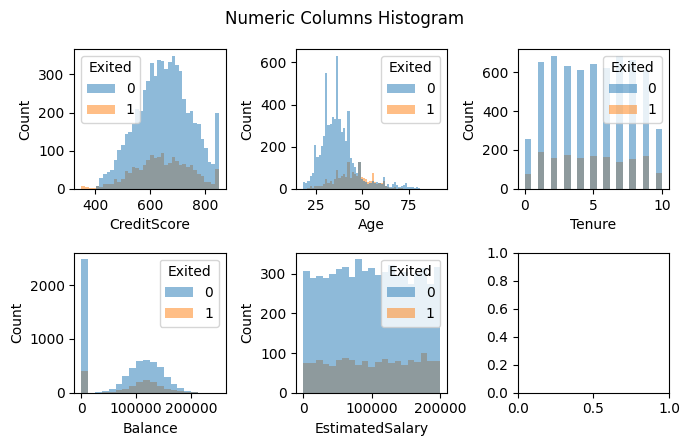
Judging from the histogram above, we can see that there doesn’t appear to be any extreme outliers. Moreover, I also cannot see if there’s any pattern between each variable and the target variable, except for Age, where older customers apppear more likely to churn. Let’s compare the churn rate of older vs younger customers (I define older customers as customers that are older than the mean):
age_avg = df_train['Age'].mean()
seniors_churn_rate = df_train[df_train['Age'] > age_avg]['Exited'].mean()
juniors_churn_rate = df_train[df_train['Age'] <= age_avg]['Exited'].mean()

print(f'Average age is {age_avg:.2f} years')
print(f'Churn rate for younger customers: {juniors_churn_rate:.2f}')
print(f'Churn rate for older customers: {seniors_churn_rate:.2f}')
Output:
Average age is 38.99 years
Churn rate for younger customers: 0.10
Churn rate for older customers: 0.34
As expected, younger customers have much lower churn rate than the older customers.
From the histogram, the variables CreditScore, Age, and Balance appear to follow the normal distribution, while EstimatedSalary appear to have a uniform distribution. Apparently, the Tenure variable has only integer values. We can also see that there are many instances where the Balance is zero. I wonder, how often do they occur?
(df_train['Balance']==0).mean()
Output:
0.36082989626296713
Pretty often, as it turns out; thirty six percent of the customers have zero balance. I expect these customers to churn more. Is it true? Let’s find out:
df_train.query('Balance==0')['Exited'].mean()
Output:
0.14063041219258746
I was wrong, apparently, as there’s only about 14% customers with zero balance that are going to churn, which is lower than the overall churn rate of 20%.
Categorical variables distributions
We’ll move on to the categorical variables. First, I’m going to plot the number of each class’ occurence in each variable:
fig, axes = create_subplots_grid(len(cat_cols), ncols=3)
fig.set_figheight(4)
fig.suptitle('Occurence of Categorical Variables')
for col,ax in zip(cat_cols, axes):
    df_train.groupby(col).size().plot.barh(ax=ax)
fig.supxlabel('Count')
plt.tight_layout()
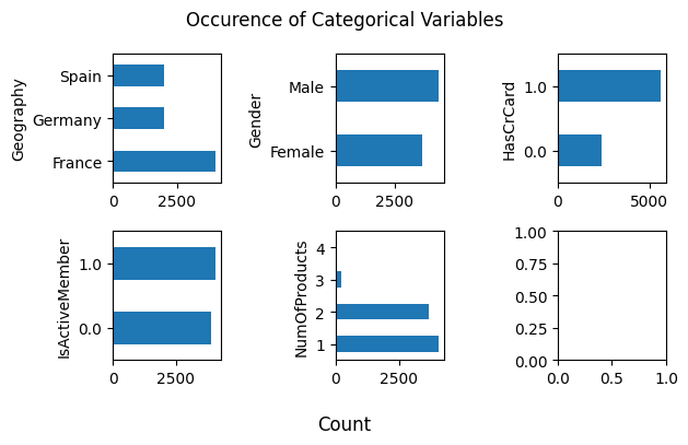
We can see that there are some class imbalance for variable Geography, HasCrCard, and NumOfProducts.
Next, I’m going to plot conditional probabilities for each unique value in each categorical variables:
fig, axes = create_subplots_grid(len(cat_cols), ncols=3)
fig.set_figheight(4)
fig.suptitle('Conditional Probability of Churning')
for col,ax in zip(cat_cols, axes):
    df_train.groupby(col)[target_col].mean().plot.barh(ax=ax)
    ax.set_xlim(0, 1)
plt.tight_layout()
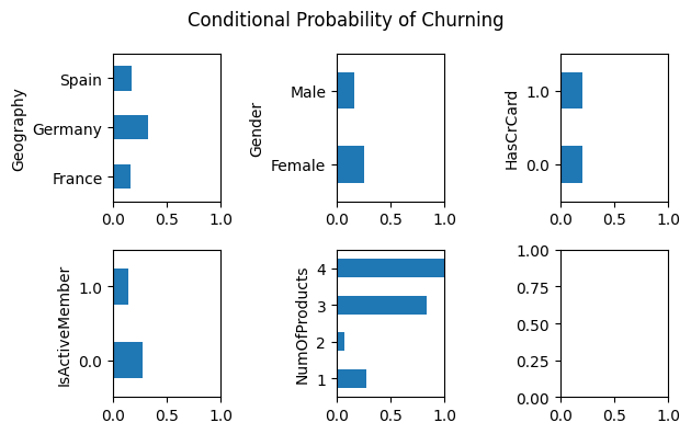
Judging from the plot above, I cannot make any conclusion relating any pattern between the categorical variables and the target variable. You may think that NumOfProducts has a clear pattern, where customers with NumOfProducts equal to four is much more likely to churn. However, we cannot make such conclusion since there’s only very few customers where the NumOfProducts is equal to four (it only occurs 0.67% of the time):
(df_train['NumOfProducts'] == 4).mean()
Output:
0.006749156355455568
Missing data & outliers
How many missing data are there?
df_train.isna().sum().sort_values()
Output:
CreditScore        0
Gender             0
Tenure             0
Balance            0
NumOfProducts      0
EstimatedSalary    0
Exited             0
Geography          1
Age                1
HasCrCard          1
IsActiveMember     1
dtype: int64
Luckily for us, there isn’t much missing data here, so we don’t have to worry too much. Later, I’ll impute the missing data with the mean (for numeric variables) and with the mode (for categorical variables).
Lastly, let’s check some statistics from each numeric variables:
df_train[num_cols].describe().T
| count | mean | std | min | 25% | 50% | 75% | max | |
|---|---|---|---|---|---|---|---|---|
| CreditScore | 8001.0 | 650.555181 | 96.610540 | 350.00 | 584.0 | 651.00 | 717.00 | 850.00 |
| Age | 8000.0 | 38.986449 | 10.577676 | 18.00 | 32.0 | 37.00 | 44.00 | 92.00 |
| Tenure | 8001.0 | 4.998625 | 2.895276 | 0.00 | 2.0 | 5.00 | 7.00 | 10.00 |
| Balance | 8001.0 | 76411.022325 | 62291.895727 | 0.00 | 0.0 | 96781.39 | 127504.57 | 250898.09 |
| EstimatedSalary | 8001.0 | 100354.149888 | 57552.877696 | 11.58 | 51219.8 | 100556.98 | 149653.81 | 199992.48 |
All variables seem to be in order.
EDA Conclusion
After doing the EDA above, I conclude that the data is already good & clean enough, given that there doesn’t appear to be invalid or outlier values, and not much missing data.
However, we still need to impute the missing data so we can train the models. The categorical variables also need to be converted to numeric by using one-hot encoding.
Preprocessing
By using the functions that I’ve written before, I’m going to transform the data in the following order:
- Impute the missing data
- Transform the categorical variables using one-hot encoding
- Split the data between predictors and the target variable
- Standardize the predictors so all of them are in the same scale (some ML models wouldn’t converge if the data are not standardized)
First, I’m going to “fit” the imputer, encoder, and standardizer objects:
num_imputer, cat_imputer = fit_imputer(
    df_train, num_cols, cat_cols
)

df_train_imp = impute_data(
    df_train, num_imputer, cat_imputer
)

ohe = fit_ohe(
    df_train_imp, cat_cols
)

df_train_ohe = transform_ohe(
    df_train_imp, ohe
)

feature_cols = [*num_cols, *ohe.get_feature_names_out()]
X_train_unscaled = df_train_ohe[feature_cols]
scaler = fit_scaler(X_train_unscaled)
Next, let’s transform all the data using the objects that I’ve just created:
preprocess_args = dict(
    num_imputer = num_imputer,
    cat_imputer = cat_imputer,
    ohe = ohe,
    scaler = scaler,
    feature_cols = feature_cols,
    target_col = target_col,
)

X_train, y_train = preprocess_data(
    df_train, **preprocess_args
)
X_valid, y_valid = preprocess_data(
    df_valid, **preprocess_args
)
X_test, y_test = preprocess_data(
    df_test, **preprocess_args
)
At this point, we already have the preprocessed data that is ready to be used for training the models.
Let’s ensure that there isn’t any missing data:
X_train.isna().sum()
Output:
CreditScore           0
Age                   0
Tenure                0
Balance               0
EstimatedSalary       0
Geography_France      0
Geography_Germany     0
Geography_Spain       0
Gender_Male           0
HasCrCard_1.0         0
IsActiveMember_1.0    0
NumOfProducts_1       0
NumOfProducts_2       0
NumOfProducts_3       0
NumOfProducts_4       0
dtype: int64
As you can see, there is no missing data anymore. You can also see that there are now additional columns created by the one-hot encoder.
Lastly, let’s check if each column has mean 0 and standard deviation of 1:
X_train.describe().T.round(2)
| count | mean | std | min | 25% | 50% | 75% | max | |
|---|---|---|---|---|---|---|---|---|
| CreditScore | 8001.0 | 0.0 | 1.0 | -3.11 | -0.69 | 0.00 | 0.69 | 2.06 |
| Age | 8001.0 | -0.0 | 1.0 | -1.98 | -0.66 | -0.19 | 0.47 | 5.01 |
| Tenure | 8001.0 | -0.0 | 1.0 | -1.73 | -1.04 | 0.00 | 0.69 | 1.73 |
| Balance | 8001.0 | 0.0 | 1.0 | -1.23 | -1.23 | 0.33 | 0.82 | 2.80 |
| EstimatedSalary | 8001.0 | -0.0 | 1.0 | -1.74 | -0.85 | 0.00 | 0.86 | 1.73 |
| Geography_France | 8001.0 | 0.0 | 1.0 | -1.01 | -1.01 | 0.99 | 0.99 | 0.99 |
| Geography_Germany | 8001.0 | 0.0 | 1.0 | -0.58 | -0.58 | -0.58 | 1.73 | 1.73 |
| Geography_Spain | 8001.0 | 0.0 | 1.0 | -0.57 | -0.57 | -0.57 | -0.57 | 1.75 |
| Gender_Male | 8001.0 | 0.0 | 1.0 | -1.09 | -1.09 | 0.92 | 0.92 | 0.92 |
| HasCrCard_1.0 | 8001.0 | -0.0 | 1.0 | -1.54 | -1.54 | 0.65 | 0.65 | 0.65 |
| IsActiveMember_1.0 | 8001.0 | 0.0 | 1.0 | -1.03 | -1.03 | 0.97 | 0.97 | 0.97 |
| NumOfProducts_1 | 8001.0 | 0.0 | 1.0 | -1.02 | -1.02 | 0.98 | 0.98 | 0.98 |
| NumOfProducts_2 | 8001.0 | 0.0 | 1.0 | -0.92 | -0.92 | -0.92 | 1.09 | 1.09 |
| NumOfProducts_3 | 8001.0 | -0.0 | 1.0 | -0.17 | -0.17 | -0.17 | -0.17 | 6.03 |
| NumOfProducts_4 | 8001.0 | 0.0 | 1.0 | -0.08 | -0.08 | -0.08 | -0.08 | 12.13 |
All seems good. Let’s move on!
Training the Model
In this section, I’m going to train the model. To achieve the best possible result, I’m going to train several models, such as logistic regression, multilayer perceptron, bagging classifier, etc. For each model, I’m also going to try several hyperparameters and choose the best one (with the aid of GridSearchCV module by scikit learn). In the end, I’m going to choose the model with the highest out-of-sample score (tested on the validation set).
What metric, then, am I going to use? This part is a little bit tricky, because the target class is pretty imbalanced (only 20% “positive” cases), and so using accuracy metric might not be the best option. Using F1 metric might sound good, since it aims to average between the precision and recall metric. However, the calculated F1 score for each model would assume the default 50% threshold (i.e. “classify as 1 if predicted probability is greater than 50%”), which might not be the optimal threshold (and the optimal threshold might be different for each model). Therefore, I decided to use the area under the ROC curve (also called AUC), which will inform me about the model performance regardless of the choice of the threshold. Later on, I will tune the optimal threshold that will minimize the dollar cost.
Below I’m specifying some inputs that are uniform for all models that I’m going to train:
score_name = 'roc_auc'
gs_config = dict(
    cv = 5,
    scoring = score_name,
)
gs_input = dict(
    X_train = X_train,
    y_train = y_train,
    X_test = X_valid,
    y_test = y_valid,
)
gs_results = {}
Next, I will train each model and find the most optimal hyperparameters. Notice how I also train a “dummy” classifier, which will act as the base-line. This classifier will only predict the mode of the target variable (zero, in this case).
Note: due to limitations of my laptop, I’m not going to do an extensive grid search (it could take hours to run). Instead, I will only search through a small selection of hyperparameters.
gs_results['DummyClassifier'] = fit_eval_cv(
    GridSearchCV(
        estimator = DummyClassifier(random_state=42),
        param_grid = {},
        **gs_config,
    ),
    **gs_input
)
gs_results['LogisticRegression'] = fit_eval_cv(
    GridSearchCV(
        estimator = LogisticRegression(solver='liblinear', random_state=42, class_weight='balanced'),
        param_grid = {
            'C': np.logspace(-5, 5, 10),
        },
        **gs_config,
    ),
    **gs_input
)
gs_results['NeuralNetwork'] = fit_eval_cv(
    GridSearchCV(
        estimator = MLPClassifier(random_state=152, hidden_layer_sizes=100),
        param_grid = {},
        **gs_config,
    ),
    **gs_input
)
gs_results['Bagging'] = fit_eval_cv(
    GridSearchCV(
        estimator = BaggingClassifier(random_state=42),
        param_grid = {
            'n_estimators': [100, 150, 200],
        },
         **gs_config,
    ),
    **gs_input
)
gs_results['DecisionTree'] = fit_eval_cv(
    GridSearchCV(
        estimator = DecisionTreeClassifier(random_state=42),
        param_grid = {
            'max_depth': [5, 10, 30],
            'min_samples_split': [2, 3, 4, 5],
            'min_samples_leaf': [10, 20, 30, 40],
        },
         **gs_config,
    ),
    **gs_input
)
gs_results['GradientBoosting'] = fit_eval_cv(
    GridSearchCV(
        estimator=GradientBoostingClassifier(random_state=42),
        param_grid={
            'n_estimators': [100, 150, 200],
        },
         **gs_config,
    ),
    **gs_input
)
Model Evaluation
Choosing the Best Model
Below is the summary of the trained models, sorted from the highest to lowest validation score:
gs_summary = pd.DataFrame(gs_results).T
gs_summary = gs_summary.sort_values('test_score', ascending=False)
gs_summary.drop('best_model', axis=1)
| test_score | f1 | roc_auc | accuracy | |
|---|---|---|---|---|
| NeuralNetwork | 0.860958 | 0.521739 | 0.860958 | 0.857 |
| GradientBoosting | 0.856939 | 0.539249 | 0.856939 | 0.865 |
| Bagging | 0.843376 | 0.545455 | 0.843376 | 0.855 |
| DecisionTree | 0.834916 | 0.442804 | 0.834916 | 0.849 |
| LogisticRegression | 0.821396 | 0.529412 | 0.821396 | 0.76 |
| DummyClassifier | 0.5 | 0.0 | 0.5 | 0.815 |
Among all tested models, the neural network model results in the highest performance with AUC of 0.861. Therefore, from here onward I’m going to use it for further analysis.
best_model = gs_summary.iloc[0]['best_model']
You might notice that the accuracy score of all models are not that great: the dummy classifier has accuracy of 0.815, while the neural network model is only slightly higher at 0.857. As we’ll see later (on later section about threshold tuning), our model could still result in lower dollar cost for the company.
Evaluating on the Test Data
To make sure that the model is going to perform out-of-sample, I’m going to test the best model’s performance on the test data:
y_test_pred_prob = best_model.predict_proba(X_test)[:, 1]
roc_auc_score(y_test, y_test_pred_prob)
Output:
0.8596494363814018
As you can see, the AUC score is 0.8596, which is very similar to the AUC score tested on the validation set.
Threshold Tuning and Cost Minimization
As I have stated previously, a neural network model will classify an observation to a particular class if the predicted probability is greater than 50% (by default). However, 50% may not be the optimal threshold, as it doesn’t consider the cost of making classification errors.
What, then, are the cost? In this case, it’s the cost of acquiring and retaining customers. Let’s assume that the company currently has $N$ customers, and this company wants to maintain this many customers. However, a certain percentage of them are going to churn. To maintain the number of customers, the company need to (1) acquire new customers (equal to the amount of churning customers), and/or (2) treat at-risk-of-churn customers to prevent them from churning. In the first case, the company need to pay the acquisition cost per customer multiplied by the number of churning customers. On the second case, the company need to pay the retention cost per customer multiplied by the number of treated customers.
Ideally, the company want to be able to identify exactly which customers are going to churn and which are not. In this case, since typically the cost of retaining customers are cheaper than the cost of acquiring customers, the company would simply pay the retaining cost to the at-risk customers only, and pay nothing to the non at-risk customers.
However, in the real world, not all customers that the company deem to be at-risk are actually at-risk of churning. In this case, some retention cost that the company has paid was actually a “waste”, since those customers are not going to churn in the first place anyway.
This is where the optimization comes in: the company should choose the threshold that will minimize the total cost.
Mathematical Explanation of the Cost
We can express the total cost $TC$ as an equation:
Using the classifier model, we are going to treat customers that are predicted positive (positive = churn in this case). Meanwhile, customers that were classified as negative but actually positive (i.e. “false negative”) would need to be acquired. So, I’m going to replace “Treated Customers” with “Predicted Positive”, and “Churning Customers” as “False Negative”:
We can divide the above equation by the number of customers $N$ to get the average total cost per customer. To simplify the equation, I will define the following:
- $ATC = \text{Total Cost} / N$ (average total cost)
- $PPR = \text{Predicted Positive} / N$ (predicted positive rate)
- $FNR = \text{False Negative} / N$ (false negative rate)
- $r = \text{Retention Cost per Customer}$
- $a = \text{Acquisitio Cost per Customer}$
The equation now becomes:
\[ATC = PPR \times r + FNR \times a\]Let $f = r / a$ be the ratio of the retention cost to the acquisition cost per customer, where $0 < f < 1$ (since retention cost is typically cheaper than the acquisition cost):
\[\begin{aligned} ATC &= PPR \times a \times f + FNR \times a\\ &= a \left( PPR \times f + FNR \right) \end{aligned}\]In the equation above, $f$ and $a$ are constants, while $PPR$ and $FNR$ depends on the model threshold $h$. I’m going to express them as a function: $PPR(h)$ and $FNR(h)$.
\[ATC(h) = a \left( PPR(h) \times f + FNR(h) \right)\]Since our task is to find $h$ that will minimize $ATC(h)$, and $a$ is a positive constant, we can simply remove $a$ from the equation, leaving us with the following optimization problem:
\[\begin{aligned} \min_h g(h) &= PPR(h) \times f + FNR(h) \\ \text{where } & 0 < h < 1 \end{aligned}\]What I’m trying to emphasize in the last part is that, to optimize the threshold $h$ that will minimize the cost, we don’t really need to know the acquisition cost $a$, only the retention cost fraction $f$. Moreover, notice that, as $h$ increases from 0 to 1, the number of predicted positive observations would decrease, while the number of false negative would increase. In other words, as $h$ increases, the retention cost would decrease (since we’re treating fewer customers), while the customer acquisition cost would increase.
Simple Example
I’m going to walk through an example and try to find the optimal threshold. Let’s assume that the fraction of retention cost to acquisition cost per customer $f$ is equal to 0.3, and the acquisition cost per customer is $100.
retention_cost_fraction = 0.3
acquisition_cost_per_customer = 100
Below I’m defining a function that will calculate the average total cost per customer:
def calc_avg_total_cost(
    acquisition_cost_per_customer: float,
    retention_cost_fraction: float,
    y_true: pd.Series,
    y_prob: pd.Series,
    threshold: float
) -> float:
    y_pred = (y_prob > threshold).astype(int)
    ppr = y_pred.mean()
    fnr = ((y_pred == 0) & (y_true == 1)).mean()
    avg_total_cost = acquisition_cost_per_customer * (
        ppr * retention_cost_fraction +
        fnr
    )
    return avg_total_cost
Now I’m going to calculate the cost for several values of threshold:
thresholds = pd.Series(np.linspace(0, 1, 20))
y_valid_pred_prob = best_model.predict_proba(X_valid)[:, 1]

avg_costs = thresholds.apply(lambda threshold: calc_avg_total_cost(
    acquisition_cost_per_customer,
    retention_cost_fraction,
    y_valid,
    y_valid_pred_prob,
    threshold
))

best_threshold = thresholds[avg_costs.argmin()]
print('Optimal threshold:', best_threshold)
print('Minimum cost: $', avg_costs.min())

plt.plot(thresholds, avg_costs, marker='.')
plt.axvline(best_threshold, c='k', ls='--', lw=1)
plt.ylabel('Average Total Cost per Customer ($)')
plt.xlabel('Threshold')
Output:
Optimal threshold: 0.21052631578947367
Minimum cost: $ 13.069999999999999
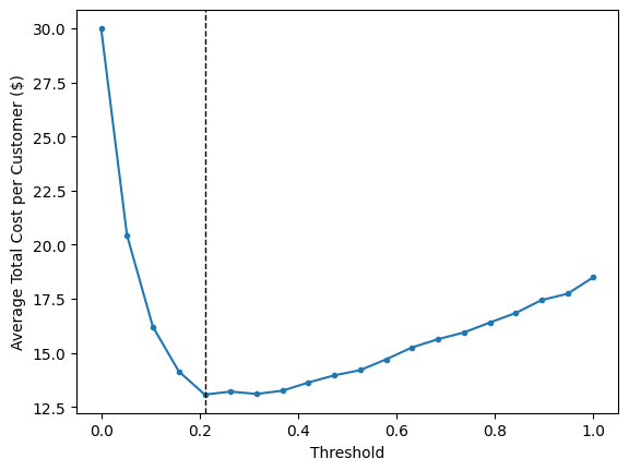
In this example, the optimum threshold is 0.21 (which is pretty far from the default threshold of 0.50), resulting in average cost of \$13 per customer. Compare it with the cost if we pay the full customer acquisition cost, which is in the right-most point in the chart above (when the threshold is equal to 1; this is also what we’d get if we use the dummy classifier, which will classify everyone as “not going to churn”):
avg_costs.iloc[-1]
Output:
18.5
The cost is \$18.5. The cost at the optimum threshold (\$13) is about 30% lower than this. To put it another way: by applying this machine learning model, the company could significantly reduce costs that it need to pay to maintain the number of customers.
Impact of Changing $f$
Let’s enrich our analysis by seeing what’s the impact of the retention cost fraction ($f$) to the choice of optimum threshold. I’m going to iterate some possible values for $f$ and find the optimum threshold and the corresponding cost at each point.
fractions = pd.Series(np.linspace(0.05, 0.95, 20))

best_thresholds = []
min_costs = []
for f in fractions:
    avg_costs_f = thresholds.apply(lambda threshold: calc_avg_total_cost(
        acquisition_cost_per_customer,
        f,
        y_valid,
        y_valid_pred_prob,
        threshold
    ))

    best_threshold_f = thresholds[avg_costs_f.argmin()]

    best_thresholds.append(best_threshold_f)
    min_costs.append(avg_costs_f.min())
Below is the plot showing the relationship between $f$ and the optimum threshold & cost.
fig, axes = plt.subplots(ncols=2)
fig.set_figwidth(10)
fig.set_figheight(4)

axes[0].plot(fractions, best_thresholds, marker='.')
axes[0].set_ylabel('Optimum Threshold')

axes[1].plot(fractions, min_costs, marker='.')
axes[1].set_ylabel('Optimum Average Cost ($)')

fig.supxlabel('Retention Cost Fraction ($f$)')
plt.tight_layout()
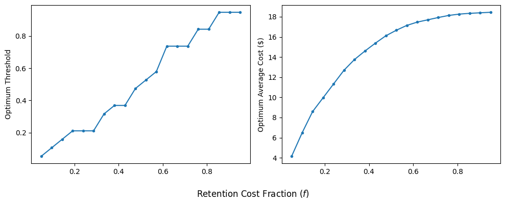
As the retention cost fraction gets closer to 1, the optimum threshold becomes higher. This should not be surprising: as the retention cost per customer increases, false positives become more expensive (i.e. the cost of unnecesarily paying retention cost to non at-risk customers), and so the model becomes more stringent (requiring higher threshold to classify customers as at-risk of churning).
And vice versa: as the retention cost per customer becomes cheaper, the model becomes less stringent. Since the retention cost is so cheap, it might be better to classify most customers as at-risk of churning.
Conclusion
In this post, I have shared how I trained a machine learning model from start to finish: doing EDA, preprocessing the data, training several models, and choosing the best one. Moreover, I have also analyzed the cost-saving impact of applying the model. After doing this exercise, I learned that a machine learning model with only moderately good performance could still significantly reduce company’s costs.
I hope you learn something new today. Cheers!