Introduction
When creating a portfolio of two stocks, the resulting standard deviations and expected returns for varying weights for each stock will result in a graph like this:
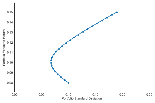
As you can see, the curve is convex to the y-axis. But why is this? Can we mathematically prove that this will always be the case?
Notations
The portfolio consists of two stocks: Stock A and Stock B. The expected returns and standard deviations for each of them are denoted as $R_A$, $R_B$, $\sigma_A$, and $\sigma_B$, respectively. The weights for each stock are denoted as $W_A$ and $W_B$, where $W_A + W_B = 1$, so $W_B = 1 - W_A$. The expected return and variance of the portfolio is
\[\begin{align*} R_p &= W_A R_A + W_B R_B \\ \sigma_p^2 &= W_A^2 \sigma_A^2 + W_B^2 \sigma_B^2 + 2 W_A W_B \cov{AB} \end{align*}\]Proving the Convexity
To answer the questions, we need to adjust our graph a bit. You see, the graph above has standard deviation as the x-axis, and expected return as the y-axis, because that is how it is usually shown. As you will see later, it is much easier to adjust the graph so the x-axis is the expected return, like this:
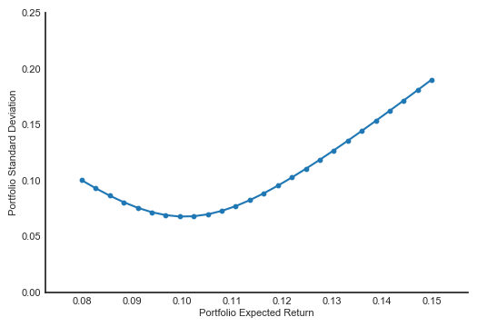
As you can immediately see, the curve appears to be quadratic. That’s what we are trying to do here: prove that the equation creating that curve is quadratic. But, what is the equation? So far we haven’t seen any function that will generate the $\sigma_p$ based on the $R_p$. That’s why first we need to find that function.
Recall that the portfolio’s variance is:
\[\begin{align*} \sigma_p^2 &= W_A^2 \sigma_A^2 + W_B^2 \sigma_B^2 + 2 W_A W_B \cov{AB} \end{align*}\]We can see that the equation above does not depend on the $R_p$. But we can also see that it depends on $W_A$, which determines the $R_p$. Arranging the equation for $R_p$ a bit, we can arrive at a nice result:
\[\begin{align*} R_p &= W_A R_A + W_B R_B \\ R_p &= W_A R_A + (1 - W_A)R_B \\ R_p &= W_A R_A + R_B - W_A R_B \\ R_p &= W_A (R_A - R_B) + R_B \\ W_A &= \frac{R_p - R_B}{R_A - R_B} \end{align*}\]We can also see that:
\[\begin{align*} W_B &= 1 - W_A \\ W_B &= 1 - \frac{R_p - R_B}{R_A - R_B} \\ W_B &= \frac{R_A - R_B}{R_A - R_B} - \frac{R_p - R_B}{R_A - R_B} \\ W_B &= \frac{R_A - R_B - (R_p - R_B)}{R_A - R_B} \\ W_B &= \frac{R_A - R_p}{R_A - R_B} \end{align*}\]Also:
\[\begin{align*} W_A W_B &= \left(\frac{R_p - R_B}{R_A - R_B}\right) \left( \frac{R_A - R_p}{R_A - R_B} \right) \\ W_A W_B &= \frac{(R_p - R_B)(R_A - R_p)}{(R_A - R_B)^2} \end{align*}\]Plugging the $W_A$, $W_B$, and $W_A W_B$ above to the equation for $\sigma_p^2$ we will see that:
The equation above can be rearranged like so:
What I just did was converting any group of variables that has nothing to do with $R_p$ into variables $X$, $Y$, and $Z$. This is mainly just for convenience, making it easier to solve the problem. In summary we have the following new variables
\[\begin{align*} X &= \frac{\sigma_A^2}{(R_A - R_B)^2} \\ Y &= \frac{\sigma_B^2}{(R_A - R_B)^2} \\ Z &= \frac{2 \cov{AB}}{(R_A - R_B)^2} \\ \end{align*}\]Now we will go back to the equation for $\sigma_p^2$:
Boom. Above you can see that the equation for $\sigma_p^2$ is quadratic with respect to the $R_p$. I have converted all of the variables that have nothing to do with $R_p$ to other variables to make it clearer:
\[\begin{align*} K &= X + Y - Z \\ L &= - 2(XR_B + YR_A - 0.5 Z R_B) \\ M &= X R_B^2 + Y R_A^2 - Z R_A R_B \\ \end{align*}\]To show that that equation for $\sigma_p^2$ is convex to the x-axis, we have to show that the coefficient that multiplies the $R_p^2$ term is always positive. In other words, $K > 0$, where $K$ is
Since the denominator is squared, then the denominator must be greater than 0 (if $R_A \neq R_B$). That left us to prove that the numerator is also greater than 0. First, remember that
\[\begin{align*} \cov{AB} = \sigma_A \sigma_B \corr{AB} \end{align*}\]Since we want to prove that the numerator is greater than zero, then we want to show that:
\[\begin{align*} \sigma_A^2 + \sigma_B^2 - 2 \cov{AB} &> 0 \\ \sigma_A^2 + \sigma_B^2 - 2 \sigma_A \sigma_B \corr{AB} &> 0 \\ \end{align*}\]For any $\sigma_A$ and $\sigma_B$, the negative term, $2 \sigma_A \sigma_B \corr{AB}$, is at the highest when $\corr{AB} = 1$ (since $-1 \leq \corr{AB} \leq 1$). If the inequality above still hold even when $\corr{AB} = 1$, then we have proven the inequality above will always be true.
For now, we will assume that $\sigma_A \neq \sigma_B$. We will express that assumption as:
\[\begin{align*} \sigma_A = \sigma_B + c \end{align*}\]Where $c$ is an arbitrary nonzero value. Then, the previous equation becomes (with $\corr{AB} = 1$):
Since the result is a squared number, then it must be positive. In other words, the following inequality is true:
\[\begin{align*} \sigma_A^2 + \sigma_B^2 - 2 \cov{AB} > 0 \end{align*}\]Recall that we want to show that the coefficient $K$
\[\begin{align*} K &= \frac{\sigma_A^2 + \sigma_B^2 - 2\cov{AB}}{(R_A - R_B)^2} \end{align*}\]is greater than zero. Since we have shown both the numerator and denominator are greater than zero, then it follows that $K$ is also greater than zero. In other words, the equation
\[\begin{align*} \sigma_p^2 &= R_p^2 K + R_p L + M \end{align*}\]always has a positive coefficient for the quadratic term $R_p^2$, which means that the equation above is convex to the x-axis, which is what we are trying to do since the beginning (in case you forgot).
\[Q. E. D.\]